Linear Regression in R, exploring a real-world dataset

#linear-regression

#oceanography

Published on Apr 24, 2023

11 min read

In this article we will explore the fundamental concepts of linear regression using a real-world dataset. We will use the Bottle Database that contains a collection of oceanographic data, including temperature, salinity, potential density and others.

This article does not aim to be a comprehensive introduction to linear regression, but rather a practical guide to get you started with the technique in real-world problems. It's important to note that although more advanced techniques may exist for certain variable relationships, we will focus on handpicking variables that are most suitable for linear regression.

Review of Linear RegressionLink to this heading

In its most general form, a regression model assumes that the response $Y$ can be expressed as a function of the predictors variables $X_1, X_2, \cdots, X_n$ plus an error term $\epsilon$ :

Y = f(X_1, X_2, \cdots, X_n) + \epsilon

In this form estimating $f$ can be quite challenging, even asuming it is smoth an continuos function. There are infinitely many possible functions that can be used, and the data alone will not tell us which one is the best. This is where linearity comes in. By assuming that the relationship between the predictors and the response is linear, we can greatly simplify the modeling process. Instead of estimating the entire function $f$ , we only need to estimate the unknown parameters in the linear regression equation:

Y = \beta_0 + \beta_1 X_1 + \beta_2 X_2 + \cdots + \beta_n X_n + \epsilon

Here $\beta_0, \beta_1, \beta_2, \beta_n$ are unknown parameters, ( $\beta_0$ is also called the intercept or bias term). Note that the predictors themselves do not have to be linear. For example, we can have a model of the form:

Y = \beta_0 + \beta_1 log(X_1) + \beta_2 X_2^2 + \beta_3 X_3 X_1 + \epsilon

which is still linear. Meanwhile:

Y = \beta_0 + \beta_1 \beta_2 X_1 + \beta_2 X_2 + \beta_3 X_3 + \epsilon

is not. Although the name implies a straight line, linear regression models can actually be quite flexible and can handle complex datasets. To capture non-linear relationships between predictors and the response variable, quadratic terms can be included in the model. Additionally, nonlinear predictors can be transformed to a linear form through suitable transformations, such as logarithmic transformation, which can linearize exponential relationships.

In practice almost all relationships could be represented or reduced to a linear form. This is why linear regression is so widespread and popular. It is a simple yet powerful technique.

Matrix representationLink to this heading

To make it easier to work with, lets present our model of a response $Y$ and $n$ predictors $X_1, X_2, \cdots, X_n$ in a tabular form:

y_1 \quad x_{11} \quad x_{12} \quad \cdots \quad x_{1n} \\ y_2 \quad x_{21} \quad x_{22} \quad \cdots \quad x_{2n} \\ \vdots \\ y_m \quad x_{m1} \quad x_{m2} \quad \cdots \quad x_{mn}

where $m$ is the number of observations or cases in the dataset. Given the actual data values, we may write the model as:

y_i = \beta_0 + \beta_1 x_{i1} + \beta_2 x_{i2} + \cdots + \beta_n x_{in} + \epsilon_i

We can write this more conveniently in matrix form as:

y = X \beta + \epsilon

where $y = (y_1, y_2, \cdots, y_m)^T$ is the response vector, $\epsilon = (\epsilon_1, \epsilon_2, \cdots, \epsilon_m)^T$ is the error vector, $\beta = (\beta_0, \beta_1, \cdots, \beta_n)^T$ is the parameter vector, and:

X = \begin{bmatrix} 1 & x_{11} & x_{12} & \cdots & x_{1n} \\ 1 & x_{21} & x_{22} & \cdots & x_{2n} \\ \vdots & \vdots & \vdots & \ddots & \vdots \\ 1 & x_{m1} & x_{m2} & \cdots & x_{mn} \end{bmatrix}

is the design matrix. Note that the first column of $X$ is all ones. This is to account for the intercept term $\beta_0$ .

Estimating the parametersLink to this heading

In order to achieve the best possible fit between our model and the data, our objective is to estimate the parameters denoted as $\beta$ . Geometrically, this involves finding the vector $\beta$ that minimizes the difference between the product $X\beta$ and the target variable $y$ . We refer to this optimal choice of $\beta$ as $\hat{\beta}$ , which is also known as the regression coefficients.

To predict the response variable, our model uses the equation $\hat{y} = X \hat{\beta}$ or, equivalently, $Hy$ , where $H$ represents an orthogonal projection matrix. The predicted values $\hat{y}$ are commonly referred to as the fitted values. On the other hand, the discrepancy between the actual response variable $y$ and the fitted response $\hat{y}$ is referred to as the residual.

Least Squares EstimationLink to this heading

Estimating $\beta$ can be approached from both a geometric and a non-geometric perspective. We define the best estimate of $\beta$ as the one that minimizes the sum of squared residuals:

\sum{\epsilon_i^2} = \epsilon^T \epsilon = (y - X \beta)^T (y - X \beta)

To find this optimal estimate, we differentiate the expression with respect to $\beta$ and set the result to zero, yielding the normal equations:

X^T X \hat{\beta} = X^T y

Interestingly, we can also derive the same result using a geometric approach:

\begin{align} \hat{\beta} &= (X^T X)^{-1} X^T y \\ X \hat{\beta} &= X (X^T X)^{-1} X^T y \\ \hat{y} &= H y \end{align}

In this context, $H = X (X^T X)^{-1} X^T$ represents the hat matrix, which serves as the orthogonal projection matrix onto the column space spanned by $X$ . While $H$ is useful for theoretical manipulations, it is typically not computed explicitly due to its size (an $n \times n$ matrix). Instead, the Moore-Penrose pseudoinverse of $X$ is employed to calculate $\hat{\beta}$ efficiently.

Note we won't explicitly calculate the inverse matrix here, but instead use the built-in R lm function.

About the datasetLink to this heading

The CalCOFI dataset is an extensive and comprehensive resource, renowned for its long-running time series spanning from 1949 to the present. With over 50,000 sampling stations, it stands as the most complete repository of oceanographic and larval fish data worldwide.

Our interest is figure out if there are variables that exhibit a linear relationship with the temperature of the water. So, let get started by loading the data getting a summary of the rows and columns.

data <- read.csv("bottle.csv")
head(data, 10)

You can check more about what means each column here.

Cleaning the dataLink to this heading

To keep this blog post concise and reader-friendly, we'll narrow our focus to five key variables: temperature, salinity, dissolved oxygen per liter, depth in meters and potential density. These variables, will be our primary points of interest. However, don't hesitate to explore any other variables that catch your attention.

To maintain data integrity, it's worth mentioning that there are some missing values within the dataset. But we can easily handle this by using the na.omit() function. It allows us to remove rows with missing values, ensuring a robust analysis.

data <- data[, c("T_degC", "Salnty", "O2ml_L", "Depthm, T_degC")]
data <- na.omit(data)

Checking for linearityLink to this heading

We want to assure that the linear model assumptions are met. This can be tested by calculating the correlation coefficients. A correlation coefficient near zero indicates that there is no linear relationship between the two variables, meanwhile, a correlation coefficient near -1 or 1 indicates that there is a strong negative or positive linear relationship. We can create a correlation matrix using the cor() function.

library(corrplot)

correlation_matrix <- cor(data)
corrplot(correlation_matrix, method = "circle")

Correlation matrix

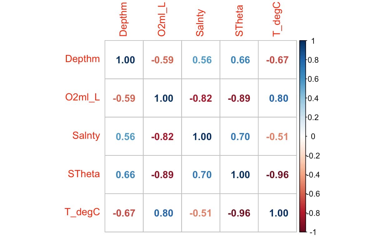
Let's narrow our attention to the variables that exhibit stronger correlation: T_degC and STheta. Since we have the flexibility to shape our exploration in this scenario, we can decide what aspects to delve into and how to approach them. However, in a real-world scenario, the variables to analyze are often dictated by the specific problem at hand.

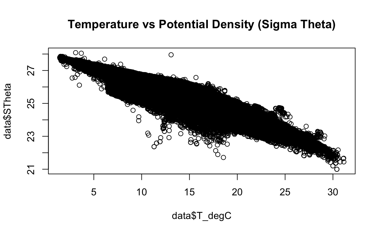
To begin our analysis, let's plot these variables and examine if there exists a linear relationship between them. This initial visualization will provide us with valuable insights into their potential connection.

plot(data$T_degC, data$STheta,
 main = "Temperature vs Potential Density (Sigma Theta)")

variable plot

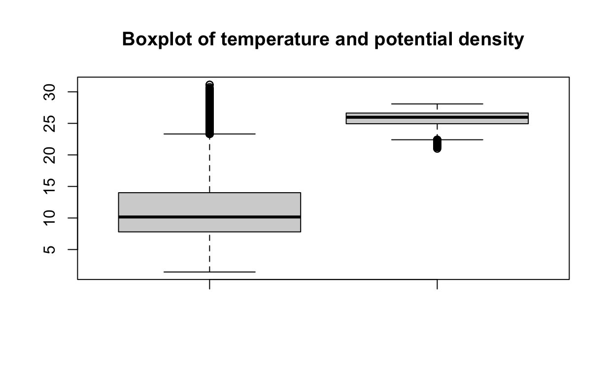
Looking for outliersLink to this heading

Outliers are data points that are far from other data points. They can be caused by experimental errors, data corruption or other anomalies. Outliers can have a large effect on the linear regression model, since they can disproportionately influence the model's fit. We can use the boxplot() function to visualize the outliers.

boxplot(data$T_degC, data$O2ml_L,
 main = "Boxplot of temperature and dissolved oxigen per litter")

By observing the plot, it appears that there may be a few data points that could be considered outliers. However, in this analysis, we will choose to retain these points. They appear to be within a reasonable range and are not significantly distant from the median. If you are interested in exploring more precise techniques for outlier detection, you can refer to this helpful resource here.

boxplot(data$T_degC, data$STheta,
 main = "Boxplot of temperature and potential density")

variable plot

Creating the modelLink to this heading

To ensure an effective evaluation of our model's performance, we will divide the data into training and testing sets. This division allows us to train our model on a subset of the data and assess its accuracy on unseen data.

For this purpose, we will allocate 80% of the data for training and reserve the remaining 20% for testing. To achieve this, we can utilize the sample() function, which enables us to randomly select the rows that will constitute the training set. This random selection ensures a representative sample and avoids bias in our model training.

training_rows <- sample(1:nrow(data), 0.8 * nrow(data))
training_data <- data[training_rows, ]
testing_data <- data[-training_rows, ]

Now we can create the linear model using the lm() function. The first argument is the formula, which is the response variable (potential density energy) followed by the predictor variable (temperature). The second argument is the dataset that is going to be used to create the model.

model <- lm(STheta ~ T_degC, data = training_data)

We can use the summary() function to get a summary of the model.

summary(model)

Call:
lm(formula = STheta ~ T_degC, data = training_data)

Residuals:
    Min      1Q  Median      3Q     Max
-3.3407 -0.1381 -0.0088  0.1076  2.0716

Coefficients:
              Estimate Std. Error t value Pr(>|t|)
(Intercept)  2.831e+01  1.020e-03   27769   <2e-16 ***
T_degC      -2.305e-01  8.712e-05   -2645   <2e-16 ***
---
Signif. codes:  0 ‘***’ 0.001 ‘**’ 0.01 ‘*’ 0.05 ‘.’ 0.1 ‘ ’ 1

Residual standard error: 0.2676 on 529012 degrees of freedom
Multiple R-squared:  0.9297,	Adjusted R-squared:  0.9297
F-statistic: 6.997e+06 on 1 and 529012 DF,  p-value: < 2.2e-16

Let first explain the output of the summary() function:

The Coefficients table shows the estimated coefficients of the linear model.
The Estimate column shows the intercept and the slope of the linear model.
The Pr(>|t|) column shows the p-value of the coefficients.
The p-value indicates if the coefficient is statistically significant.
The Residual standard error is the standard deviation of the residuals.
The Multiple R-squared is the proportion of the variance in the response variable that is explained by the predictors.
The Adjusted R-squared is the R-squared adjusted for the number of predictors in the model.
The F-statistic is the ratio of the mean regression sum of squares divided by the mean error sum of squares.
The p-value of the F-statistic indicates if the model is statistically significant.

Based on the p-value of the coefficients, we can conclude that the intercept and the slope are statistically significant.

Making predictionsLink to this heading

We can use the predict() function to make predictions on the testing set. The first argument is the model, the second argument is the dataset that is going to be used to make the predictions. The predict() function returns a vector of predictions.

predictions <- predict(model, testing_data)

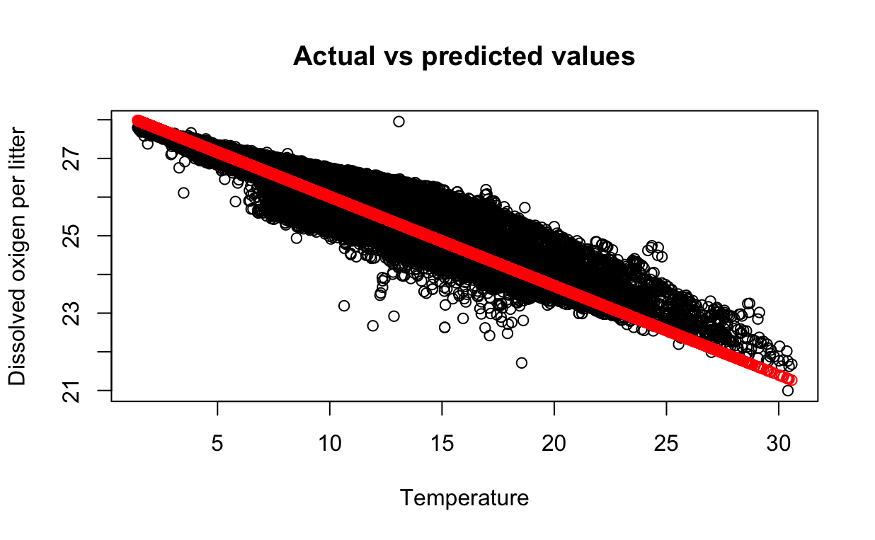
We can use the plot() function to plot the actual values vs the predicted values.

plot(testing_data$T_degC, testing_data$STheta,
  main = "Actual vs predicted values",
  xlab = "Temperature", ylab = "Potential density")

points(testing_data$T_degC, predictions, col = "red")

The red points are the predicted values and the blue points are the actual values. We can see that the predicted values are close to the actual values.

variable plot

ReferencesLink to this heading

Faraway, Julian J. Linear Models with Python. CRC Press, 2021.
Heumann, Christian, and Micheal Schomaker Shalabh. Introduction to statistics and data analysis. Springer, 2016.